Factors

R has a special data class, called factor, to deal with categorical data that you may encounter when creating plots or doing statistical analyses.

Factors represent categorical data. They are stored as integers associated with labels and they can be ordered (ordinal) or unordered (nominal). Factors create a structured relation between the different levels (values) of a categorical variable, such as days of the week or responses to a question in a survey. This can make it easier to see how one element relates to the other elements in a column. While factors look (and often behave) like character vectors, they are actually treated as integer vectors by R. So you need to be very careful when treating them as strings.

Once created, factors can only contain a predefined set of values, known as levels. By default, R always sorts levels in alphabetical order. For instance, if you have a factor with 2 levels:

respondent_floor_type <-factor(c("earth", "cement", "cement", "earth"))

R will assign 1 to the level “cement” and 2 to the level “earth” (because c comes before e, even though the first element in this vector is “earth”). You can see this by using the function levels() and you can find the number of levels using nlevels():

levels(respondent_floor_type) 
[1] "cement" "earth" 
nlevels(respondent_floor_type) 
[1] 2 

Sometimes, the order of the factors does not matter. Other times you might want to specify the order because it is meaningful (e.g., “low”, “medium”, “high”). It may improve your visualization, or it may be required by a particular type of analysis. Here, one way to reorder our levels in the respondent_floor_type vector would be:

respondent_floor_type # current order 
[1] earth cement cement earth 
Levels: cement earth 
respondent_floor_type <- factor(respondent_floor_type, levels = c("earth", "cement")) respondent_floor_type # after re-ordering 
[1] earth cement cement earth 
Levels: earth cement 

In R’s memory, these factors are represented by integers (1, 2), but are more informative than integers because factors are self describing: “cement”, “earth” is more descriptive than 1, and 2. It is particularly helpful when there are many levels. It also makes renaming levels easier. Let’s say we made a mistake and need to recode “cement” to “brick”.

levels(respondent_floor_type) 
[1] "earth" "cement" 
levels(respondent_floor_type)[2] <- "brick" 
levels(respondent_floor_type) 
[1] "earth" "brick" 
respondent_floor_type 
[1] earth brick brick earth 
Levels: earth brick 

So far, your factor is unordered, like a nominal variable. R does not know the difference between a nominal and an ordinal variable. You make your factor an ordered factor by using the ordered=TRUE option inside your factor function. Note how the reported levels changed from the unordered factor above to the ordered version below. Ordered levels use the less than sign < to denote level ranking.

respondent_floor_type_ordered <- factor(respondent_floor_type, ordered=TRUE) respondent_floor_type_ordered # after setting as ordered factor 
[1] earth brick brick earth 
Levels: earth < brick 

Converting factors

If you need to convert a factor to a character vector, you use as.character(x).

as.character(respondent_floor_type) 
[1] "earth" "brick" "brick" "earth"

Converting factors where the levels appear as numbers (such as concentration levels, or years) to a numeric vector is a little trickier. The as.numeric() function returns the index values of the factor, not its levels, so it will result in an entirely new (and unwanted in this case) set of numbers. One method to avoid this is to convert factors to characters, and then to numbers. Another method is to use the levels() function. Compare:

year_fct <-factor(c(1990, 1983, 1977, 1998, 1990)) 
as.numeric(year_fct) # Wrong! And there is no warning... 
[1] 3 2 1 4 3 
as.numeric(as.character(year_fct)) # Works... 
[1] 1990 1983 1977 1998 1990 as.numeric(levels(year_fct))[year_fct] # The recommended way. 
[1] 1990 1983 1977 1998 1990 

Notice that in the recommended levels() approach, three important steps occur:

• We obtain all the factor levels using levels(year_fct)
• We convert these levels to numeric values using as.numeric(levels(year_fct))
• We then access these numeric values using the underlying integers of the vector year_fct inside the square brackets

Renaming factors

When your data is stored as a factor, you can use the plot() function to get a quick glance at the number of observations represented by each factor level. Let’s extract the memb_assoc column from our data frame, convert it into a factor, and use it to look at the number of interview respondents who were or were not members of an irrigation association:

## create a vector from the data frame column "memb_assoc" 
memb_assoc <-interviews$memb_assoc 
## convert it into a factor 
memb_assoc <-as.factor(memb_assoc) 
## let's see what it looks like 
memb_assoc 
[1] <NA> yes <NA> <NA> <NA> <NA> no yes no no <NA> yes no <NA> yes 
[16] <NA> <NA> <NA> <NA> <NA> no <NA> <NA> no no no <NA> no yes <NA> 
[31] <NA> yes no yes yes yes <NA> yes <NA> yes <NA> no no <NA> no 
[46] no yes <NA> <NA> yes <NA> no yes no <NA> yes no no <NA> no 
[61] yes <NA> <NA> <NA> no yes no no no no yes <NA> no yes <NA> 
[76]  <NA>  yes  no  no  yes  no  no  yes  no  yes  no  no  
<NA>  yes  yes  
[91]  yes  yes  yes  no  no  no  no  yes  no  no  yes  yes  no  
<NA>  no  
[106]  no  <NA>  no  no  <NA>  no  <NA>  <NA>  no  no  no  no  yes  
no  no  
[121]  no  no  no  no  no  no  no  no  no  yes  <NA>  
Levels:  no  yes  
##  bar  plot  of  the  number  of  interview  respondents  who  were  
##  members  of  irrigation  association:  
plot(memb_assoc) 

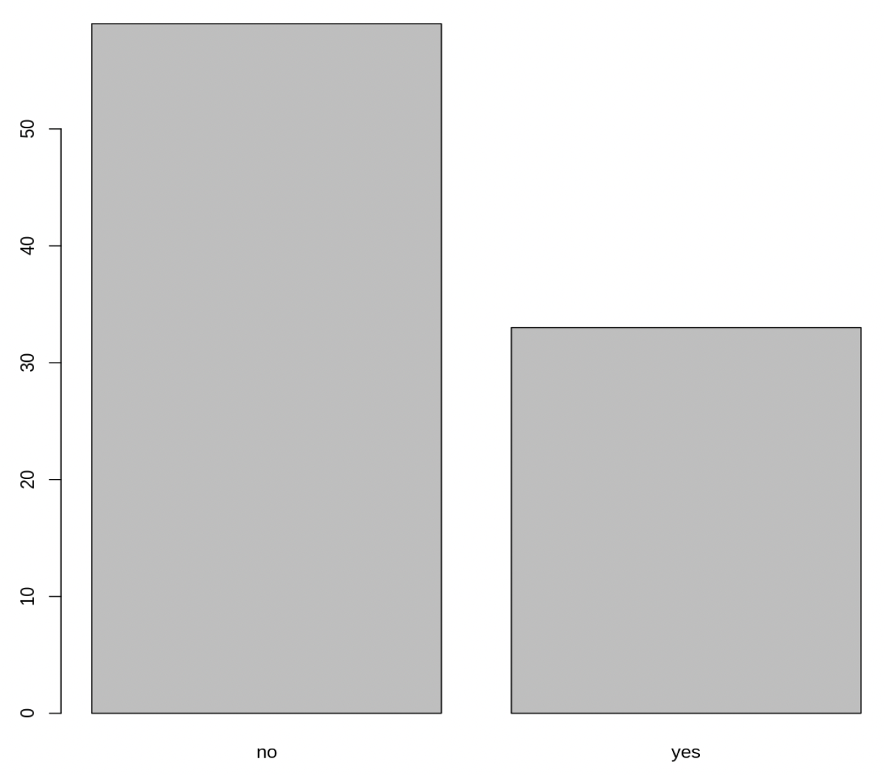
Looking at the plot compared to the output of the vector, we can see that in addition to “no’s” and “yes’s”, there are some respondents for which the information about whether they were part of an irrigation association hasn’t been recorded and encoded as missing data. They do not appear on the plot. Let’s encode them differently so they can be counted and visualized in our plot.

## Let's recreate the vector from the data frame column "memb_assoc" 
memb_assoc <-interviews$memb_assoc 
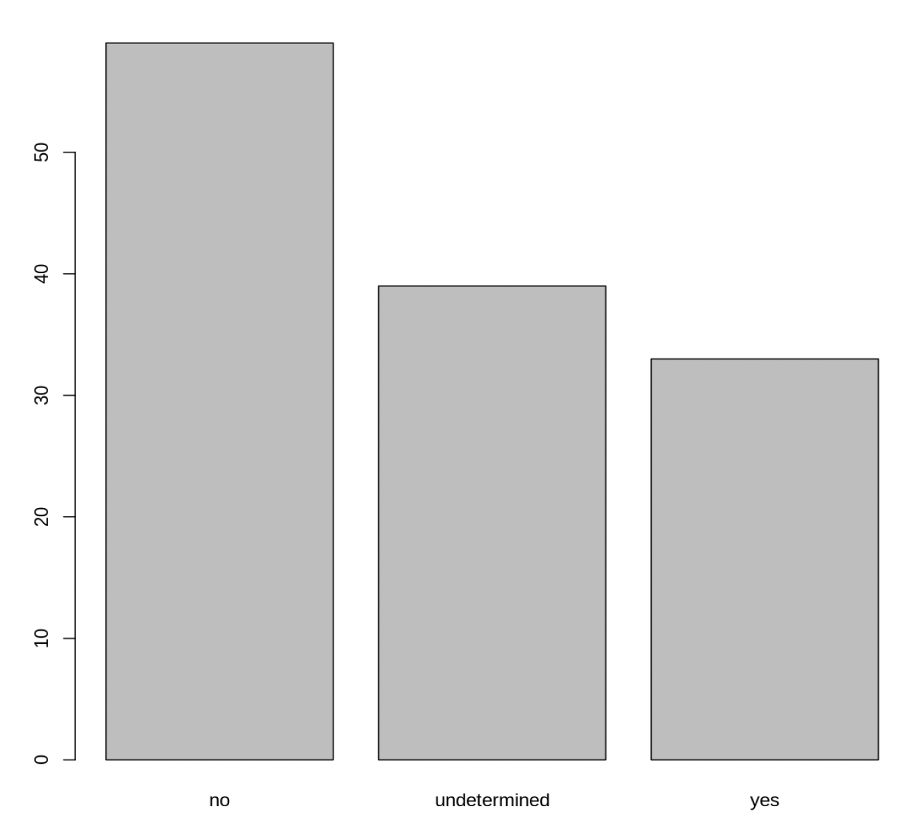
## replace the missing data with "undetermined" 
memb_assoc[is.na(memb_assoc)] <-"undetermined" 
## convert it into a factor 
memb_assoc <-as.factor(memb_assoc) 
## let's see what it looks like 
memb_assoc 
[1] undetermined yes undetermined undetermined undetermined 
[6] undetermined no yes no no 
[11] undetermined yes no undetermined yes 
[16] undetermined undetermined undetermined undetermined undetermined 
[21] no undetermined undetermined no no 
[26] no undetermined no yes undetermined 
[31] undetermined yes no yes yes 
[36] yes undetermined yes undetermined yes 
[41] undetermined no no undetermined no 
[46] no yes undetermined undetermined yes 
[51] undetermined no yes no undetermined 
[56] yes no no undetermined no 
[61] yes undetermined undetermined undetermined no 
[66] yes no no no no 
[71] yes undetermined no yes undetermined 
[76] undetermined yes no no yes 
[81] no no yes no yes 
[86] no no undetermined yes yes 
[91] yes yes yes no no 
[96] no no yes no no 
[101] yes yes no undetermined no 
[106] no undetermined no no undetermined 
[111] no undetermined undetermined no no 
[116] no no yes no no 
[121] no no no no no 
[126] no no no no yes 
[131] undetermined Levels: no undetermined yes 
## bar plot of the number of interview respondents who were ## members of irrigation association: 
plot(memb_assoc) 

Exercise

• Rename the levels of the factor to have the first letter in uppercase: “No”, ”Undetermined”, and “Yes”.
• Now that we have renamed the factor level to “Undetermined”, can you recreate the barplot such that “Undetermined” is last (after “Yes”)?

Key Points

• Use read_csv to read tabular data in R.
• Use factors to represent categorical data in R.