Indexing, Slicing and Subsetting DataFrames in Python
Objectives
- Describe what 0-based indexing is.
- Manipulate and extract data using column headings and index locations.
- Employ slicing to select sets of data from a DataFrame.
- Employ label and integer-based indexing to select ranges of data in a dataframe.
- Reassign values within subsets of a DataFrame.
- Create a copy of a DataFrame.
- Query / select a subset of data using a set of criteria using the following operators:
==,!=,>,<,>=,<=. - Locate subsets of data using masks.
- Describe BOOLEAN objects in Python and manipulate data using BOOLEANs.
Questions
- How can I access specific data within my data set?
- How can Python and Pandas help me to analyse my data?
In This Lesson
In the first episode of this lesson, we read a CSV file into a pandas’ DataFrame. We learned how to:
- save a DataFrame to a named object,
- perform basic math on data,
- calculate summary statistics, and
- create plots based on the data we loaded into pandas.
In this lesson, we will explore ways to access different parts of the data using:
- indexing,
- slicing, and
- subsetting.
Loading our data
We will continue to use the surveys dataset that we worked with in the last episode. Let’s reopen and read in the data again:
# Make sure pandas is loaded
import pandas as pd

# Read in the survey CSV
surveys_df = pd.read_csv("data/surveys.csv")
Indexing and Slicing in Python
We often want to work with subsets of a DataFrame object. There are different ways to accomplish this including: using labels (column headings), numeric ranges, or specific x,y index locations.
Selecting data using Labels (Column Headings)
We use square brackets [] to select a subset of a Python object. For example, we can select all data from a column named species_id from the surveys_df DataFrame by name. There are two ways to do this:
# TIP: use the .head() method we saw earlier to make output shorter
# Method 1: select a 'subset' of the data using the column name
surveys_df['species_id']

# Method 2: use the column name as an 'attribute'; gives the same output
surveys_df.species_id
We can also create a new object that contains only the data within the species_id column as follows:
# Creates an object, surveys_species, that only contains the `species_id` column
surveys_species = surveys_df['species_id']
We can pass a list of column names too, as an index to select columns in that order. This is useful when we need to reorganize our data.
NOTE: If a column name is not contained in the DataFrame, an exception (error) will be raised.
# Select the species and plot columns from the DataFrame
surveys_df[['species_id', 'plot_id']]

# What happens when you flip the order?
surveys_df[['plot_id', 'species_id']]

# What happens if you ask for a column that doesn't exist?
surveys_df['speciess']
Python tells us what type of error it is in the traceback, at the bottom it says KeyError: 'speciess' which means that speciess is not a valid column name (nor a valid key in the related Python data type dictionary).
Extracting Range based Subsets: Slicing
Reminder
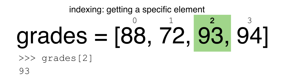
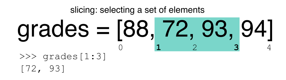
Let’s remind ourselves that Python uses 0-based indexing. This means that the first element in an object is located at position 0. This is different from other tools like R and Matlab that index elements within objects starting at 1.
# Create a list of numbers:
a = [1, 2, 3, 4, 5]
Slicing Subsets of Rows in Python
Slicing using the [] operator selects a set of rows and/or columns from a DataFrame. To slice out a set of rows, you use the following syntax: data[start:stop]. When slicing in pandas the start bound is included in the output. The stop bound is one step BEYOND the row you want to select. So if you want to select rows 0, 1 and 2 your code would look like this:
# Select rows 0, 1, 2 (row 3 is not selected)
surveys_df[0:3]
The stop bound in Python is different from what you might be used to in languages like Matlab and R.
# Select the first 5 rows (rows 0, 1, 2, 3, 4)
surveys_df[:5]

# Select the last element in the list
# (the slice starts at the last element, and ends at the end of the list)
surveys_df[-1:]
We can also reassign values within subsets of our DataFrame.
But before we do that, let’s look at the difference between the concept of copying objects and the concept of referencing objects in Python.
Copying Objects vs Referencing Objects in Python
Let’s start with an example:
# Using the '=' operator
ref_surveys_df = surveys_df

# Using the 'copy() method'
true_copy_surveys_df = surveys_df.copy()
You might think that the code ref_surveys_df = surveys_df creates a fresh distinct copy of the surveys_df DataFrame object. However, using the = operator in the simple statement y = x does not create a copy of our DataFrame. Instead, y = x creates a new variable y that references the same object that x refers to. To state this another way, there is only one object (the DataFrame), and both x and y refer to it.
In contrast, the copy() method for a DataFrame creates a true copy of the DataFrame.
Let’s look at what happens when we reassign the values within a subset of the DataFrame that references another DataFrame object:
# Assign the value `0` to the first three rows of data in the DataFrame
ref_surveys_df[0:3] = 0
Let’s try the following code:
# ref_surveys_df was created using the '=' operator
ref_surveys_df.head()

# true_copy_surveys_df was created using the copy() function
true_copy_surveys_df.head()

# surveys_df is the original dataframe
surveys_df.head()
What is the difference between these three dataframes?
When we assigned the first 3 rows the value of 0 using the ref_surveys_df DataFrame, the surveys_df DataFrame is modified too. Remember we created the reference ref_surveys_df object above when we did ref_surveys_df = surveys_df. Remember surveys_df and ref_surveys_df refer to the same exact DataFrame object. If either one changes the object, the other will see the same changes to the reference object.
However - true_copy_surveys_df was created via the copy() function. It retains the original values for the first three rows.
To review and recap:
-
Copy uses the dataframe’s
copy()methodtrue_copy_surveys_df = surveys_df.copy() -
A Reference is created using the
=operatorref_surveys_df = surveys_df
Okay, that’s enough of that. Let’s create a brand new clean dataframe from the original data CSV file.
surveys_df = pd.read_csv("data/surveys.csv")
Slicing Subsets of Rows and Columns in Python
We can select specific ranges of our data in both the row and column directions using either label or integer-based indexing.
-
ilocis primarily an integer based indexing counting from 0. That is, you specify rows and columns using a number. Thus, the first row is row 0, the second column is column 1, etc. -
locis primarily a label based indexing where you can refer to rows and columns by their name. E.g., column ‘month’. Note that integers may be used, but they are interpreted as a label.
To select a subset of rows and columns from our DataFrame, we can use the iloc method. For example, we can select the first three rows with the month, day and year (columns 2, 3 and 4 if we start counting at 1), like this:
# iloc[row slicing, column slicing]
surveys_df.iloc[0:3, 1:4]
which gives the output
   month  day  year
0      7   16  1977
1      7   16  1977
2      7   16  1977
Notice that we asked for a slice from 0:3. This yielded 3 rows of data. When you ask for 0:3, you are actually telling Python to start at index 0 and select rows 0, 1, 2 up to but not including 3.
Let’s explore some other ways to index and select subsets of data:
# Select all columns for the first three rows
surveys_df.iloc[0:3, :]

# Select all columns for rows of index values 0 and 10
surveys_df.iloc[[0, 10], :]
Now let’s explore what the loc method does
# What does this do?
surveys_df.loc[0, ['species_id', 'plot_id', 'weight']]

# What happens when you type the code below?
surveys_df.loc[[0, 10, 35549], :]
NOTE: Labels must be found in the DataFrame or you will get a KeyError.
Indexing by labels loc differs from indexing by integers iloc. With loc, both the start bound and the stop bound are inclusive. When using loc, integers can be used, but the integers refer to the index label and not the position. For example, using loc and select 1:4 will get a different result than using iloc to select rows 1:4.
We can also select a specific data value using a row and column location within the DataFrame and iloc indexing:
# Syntax for iloc indexing to finding a specific data element
dat.iloc[row, column]
In this iloc example,
surveys_df.iloc[2, 6]
gives the output
'F'
Remember that Python indexing begins at 0. So, the index location [2, 6] selects the element that is 3 rows down and 7 columns over in the DataFrame.
It is worth noting that rows are selected when using loc with a single list of labels (or iloc with a single list of integers). However, unlike loc or iloc, indexing a data frame directly with labels will select columns (e.g. surveys_df[['species_id', 'plot_id', 'weight']]), while ranges of integers will select rows (e.g. surveys_df[0:13]). Direct indexing of rows is redundant with using iloc, and direct indexing will raise a KeyError if a single integer or list is used; the error will also occur if index labels are used without loc (or column labels used with it). A useful rule of thumb is the following: integer-based slicing is best done with iloc and will avoid errors (and is generally consistent with indexing of Numpy arrays), label-based slicing of rows is done with loc, and slicing of columns by directly indexing column names.
Challenge - Range
- What happens when you execute:
surveys_df[0:3]surveys_df[0]surveys_df[0:1]surveys_df[:5]surveys_df[:-1]
- What happens when you call:
surveys_df.iloc[0:1]surveys_df.iloc[0]surveys_df.iloc[:4, :]surveys_df.iloc[0:4, 1:4]surveys_df.loc[0:4, 1:4]
- How are the last two commands different?
Solution
Selection Challenges
-
surveys_df[0:3]returns the first three rows of the DataFrame:
         record_id  month  day  year  plot_id species_id sex  hindfoot_length  weight
   0          1      7   16  1977        2         NL   M             32.0     NaN
   1          2      7   16  1977        3         NL   M             33.0     NaN
   2          3      7   16  1977        2         DM   F             37.0     NaN
surveys_df[0]results in a ‘KeyError’, since direct indexing of a row is redundant withiloc.surveys_df[0:1]can be used to obtain only the first row.surveys_df[:5]slices from the first row to the fifth:
      record_id  month  day  year  plot_id species_id sex  hindfoot_length  weight
   0          1      7   16  1977        2         NL   M             32.0     NaN
   1          2      7   16  1977        3         NL   M             33.0     NaN
   2          3      7   16  1977        2         DM   F             37.0     NaN
   3          4      7   16  1977        7         DM   M             36.0     NaN
   4          5      7   16  1977        3         DM   M             35.0     NaN
surveys_df[:-1]provides everything except the final row of the DataFrame. You can use negative index numbers to count backwards from the last entry.surveys_df.iloc[0:1]returns the first rowsurveys_df.iloc[0]returns the first row as a named listsurveys_df.iloc[:4, :]returns all columns of the first four rowssurveys_df.iloc[0:4, 1:4]selects specified columns of the first four rowssurveys_df.loc[0:4, 1:4]results in a ‘TypeError’ - see below.- While
ilocuses integers as indices and slices accordingly,locworks with labels. It is like accessing values from a dictionary, asking for the key names. Column names 1:4 do not exist, so the call tolocabove results in an error. Check also the difference betweensurveys_df.loc[0:4]andsurveys_df.iloc[0:4]. Then finally, trysurveys_df.loc[0:4, 'month':'year'], to see how to use a range of column labels.
- While
Subsetting Data using Criteria
We can also select a subset of our data using criteria. For example, we can select all rows that have a year value of 2002:
surveys_df[surveys_df.year == 2002]
Which produces the following output:
record_id  month  day  year  plot_id species_id  sex  hindfoot_length  weight
33320      33321      1   12  2002        1         DM    M     38      44
33321      33322      1   12  2002        1         DO    M     37      58
33322      33323      1   12  2002        1         PB    M     28      45
33323      33324      1   12  2002        1         AB  NaN    NaN     NaN
33324      33325      1   12  2002        1         DO    M     35      29
...
35544      35545     12   31  2002       15         AH  NaN    NaN     NaN
35545      35546     12   31  2002       15         AH  NaN    NaN     NaN
35546      35547     12   31  2002       10         RM    F     15      14
35547      35548     12   31  2002        7         DO    M     36      51
35548      35549     12   31  2002        5        NaN  NaN    NaN     NaN

[2229 rows x 9 columns]
Or we can select all rows that do not contain the year 2002:
surveys_df[surveys_df.year != 2002]
We can define sets of criteria too:
surveys_df[(surveys_df.year >= 1980) & (surveys_df.year <= 1985)]
Python Syntax Cheat Sheet
We can use the syntax below when querying data by criteria from a DataFrame. Experiment with selecting various subsets of the “surveys” data.
- Equals:
== - Not equals:
!= - Greater than:
> - Less than:
< - Greater than or equal to:
>= - Less than or equal to:
<=
Challenge - Queries
- Select a subset of rows in the
surveys_dfDataFrame that contain data from the year 1999 and that contain weight values less than or equal to 8. How many rows did you end up with? What did your neighbor get? -
You can use the
isincommand in Python to query a DataFrame based upon a list of values as follows:surveys_df[surveys_df['species_id'].isin([listGoesHere])]Use the
isinfunction to find all plots that contain particular species in the “surveys” DataFrame. How many records contain these values? - Experiment with other queries. Create a query that finds all rows with a weight value greater than or equal to 0.
- The
~symbol in Python can be used to return the OPPOSITE of the selection that you specify. It is equivalent to is not in. Write a query that selects all rows with sex NOT equal to ‘M’ or ‘F’ in the “surveys” data.
Solution
-
surveys_df[(surveys_df["year"] == 1999) & (surveys_df["weight"] <= 8)]
          record_id  month  day  year  plot_id species_id sex  hindfoot_length  weight
   29082      29083      1   16  1999       21         RM   M             16.0     8.0
   29196      29197      2   20  1999       18         RM   M             18.0     8.0
   29421      29422      3   15  1999       16         RM   M             15.0     8.0
   29903      29904     10   10  1999        4         PP   M             20.0     7.0
   29905      29906     10   10  1999        4         PP   M             21.0     4.0
If you are only interested in how many rows meet the criteria, the sum of True values could be used instead:
sum((surveys_df["year"] == 1999) & (surveys_df["weight"] <= 8))
5
-
For example, using
PBandPL:surveys_df[surveys_df['species_id'].isin(['PB', 'PL'])]['plot_id'].unique()array([ 1, 10, 6, 24, 2, 23, 19, 12, 20, 22, 3, 9, 14, 13, 21, 7, 11, 15, 4, 16, 17, 8, 18, 5])surveys_df[surveys_df['species_id'].isin(['PB', 'PL'])]['plot_id'].unique().shape(24,) surveys_df[surveys_df["weight"] >= 0]-
surveys_df[~surveys_df["sex"].isin(['M', 'F'])]
          record_id  month  day  year  plot_id species_id  sex  hindfoot_length  weight
   13            14      7   16  1977        8         DM  NaN              NaN     NaN
   18            19      7   16  1977        4         PF  NaN              NaN     NaN
   33            34      7   17  1977       17         DM  NaN              NaN     NaN
   56            57      7   18  1977       22         DM  NaN              NaN     NaN
   76            77      8   19  1977        4         SS  NaN              NaN     NaN
   ...          ...    ...  ...   ...      ...        ...  ...              ...     ...
   35527      35528     12   31  2002       13         US  NaN              NaN     NaN
   35543      35544     12   31  2002       15         US  NaN              NaN     NaN
   35544      35545     12   31  2002       15         AH  NaN              NaN     NaN
   35545      35546     12   31  2002       15         AH  NaN              NaN     NaN
   35548      35549     12   31  2002        5        NaN  NaN              NaN     NaN

   [2511 rows x 9 columns]
Using masks to identify a specific condition
A mask can be useful to locate where a particular subset of values exist or don’t exist - for example, NaN, or “Not a Number” values. To understand masks, we also need to understand BOOLEAN objects in Python.
Boolean values include True or False. For example,
# Set x to 5
x = 5

# What does the code below return?
x > 5

# How about this?
x == 5
When we ask Python whether x is greater than 5, it returns False. This is Python’s way to say “No”. Indeed, the value of x is 5, and 5 is not greater than 5.
To create a boolean mask:
- Set the True / False criteria (e.g.
values > 5 = True) - Python will then assess each value in the object to determine whether the value meets the criteria (True) or not (False).
- Python creates an output object that is the same shape as the original object, but with a
TrueorFalsevalue for each index location.
Let’s try this out. Let’s identify all locations in the survey data that have null (missing or NaN) data values. We can use the isnull method to do this. The isnull method will compare each cell with a null value. If an element has a null value, it will be assigned a value of True in the output object.
pd.isnull(surveys_df)
A snippet of the output is below:
      record_id  month    day   year plot_id species_id    sex  hindfoot_length weight
0         False  False  False  False   False      False  False   False      True
1         False  False  False  False   False      False  False   False      True
2         False  False  False  False   False      False  False   False      True
3         False  False  False  False   False      False  False   False      True
4         False  False  False  False   False      False  False   False      True

[35549 rows x 9 columns]
To select the rows where there are null values, we can use the mask as an index to subset our data as follows:
# To select just the rows with NaN values, we can use the 'any()' method
surveys_df[pd.isnull(surveys_df).any(axis=1)]
Note that the weight column of our DataFrame contains many null or NaN values. We will explore ways of dealing with this in the next episode on Data Types and Formats.
We can run isnull on a particular column too. What does the code below do?
# What does this do?
empty_weights = surveys_df[pd.isnull(surveys_df['weight'])]['weight']
print(empty_weights)
Let’s take a minute to look at the statement above. We are using the Boolean object pd.isnull(surveys_df['weight']) as an index to surveys_df. We are asking Python to select rows that have a NaN value of weight.
Take Home Challenge - Putting it all together
- Create a new DataFrame that only contains observations with sex values that are not female or male. Print the number of rows in this new DataFrame. Verify the result by comparing the number of rows in the new DataFrame with the number of rows in the surveys DataFrame where sex is null.
- Create a new DataFrame that contains only observations that are of sex male or female and where weight values are greater than 0. Create a stacked bar plot of average weight by plot with male vs female values stacked for each plot.
Solution
-
   new = surveys_df[~surveys_df['sex'].isin(['M', 'F'])].copy()
   print(len(new))
2511
sum(surveys_df['sex'].isnull()) == len(new)
True
-
   # selection of the data with isin
   stack_selection = surveys_df[(surveys_df['sex'].isin(['M', 'F'])) &
             surveys_df["weight"] > 0.][["sex", "weight", "plot_id"]]
   # calculate the mean weight for each plot id and sex combination:
   stack_selection = stack_selection.groupby(["plot_id", "sex"]).mean().unstack()
   # and we can make a stacked bar plot from this:
   stack_selection.plot(kind='bar', stacked=True)
Key Points
- In Python, portions of data can be accessed using indices, slices, column headings, and condition-based subsetting.
- Python uses 0-based indexing, in which the first element in a list, tuple or any other data structure has an index of 0.
- Pandas enables common data exploration steps such as data indexing, slicing and conditional subsetting.
Acknowledgment
The material for this workshop series was created from the Data Analysis and Visualization in Python for Ecologists curriculum developed by The Data Carpentry Foundation of The Carpentries licensed under CC-BY 4.0